In an insightful recent JD Supra® article, Feltman-Frank and coauthors discuss the potential risks that companies face if they do not carefully consider the environmental justice (EJ) landscape within which they operate (“Client Alert: Embracing Environmental Justice Initiatives to Advance Corporate Objectives” May 4, 2023). The article presents a case in which a permit for a new investment in Louisiana was vacated because the Louisiana Department of Environmental Quality deemed the EJ analysis arbitrary and capricious. The authors also note that the U.S. Environmental Protection Agency’s strategic plan for fiscal years 2022–2026 (https://www.epa.gov/planandbudget/strategicplan) emphasizes “identifying remedies…that offer tangible benefits” to affected communities, and encourages “supplemental environmental projects that are tied to addressing adverse environmental impacts…”

The authors urge companies to “…consider how to mitigate potential issues ahead of time” using tools for “…analyzing health, social, and economic effects of a specific project.” They proceed to recommend that firms facing potential obstacles to investment plans complete an EJ analysis, “…which should consider cumulative impacts….” An EJ analysis can answer important questions such as : Who is being affected by the action? How, and by how much? Compared to whom? Can we mitigate the effects and, if so, how? To fail to do so, the authors conclude, “…may result in significant hurdles to project development.”

We wholeheartedly agree. But the article’s recommendations prompt important questions. How would a reasoned EJ analysis measure the amount of injustice to determine if a SEP offsets an impact? There are many ways to answer that question, and some could be judged better than others if one has a clear view of what “better” means in this setting. When embarking on an approach such as that suggested by Feltman-Frank and coauthors, considerable care should be devoted to the measurement task. Clearly, a full treatment is beyond our scope here, but a simple example can shed light on one general approach.

Consider a simple scenario to exhibit the issues involved. There are two communities, each with three inhabitants, and four outcomes of economic and social processes that cumulatively affect the well-being of individuals and on which decision-makers can act: 1) acres of public open space within 10 minutes travel time from home (PARKS), 2) annual days with a wet bulb temperature above 85^oF (HEAT), 3) annual days with particulate matter 2.5 below 15 μgm³ (AIR), and 4) annual household income in thousands of dollars (INCOME).

“Achievement” on these outcomes can be tabulated in a matrix, for example, as follows:

Table 1. Individuals’ Levels of Achievement on Indicators of Well-being

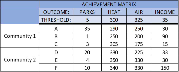
The “thresholds” in this example are hypothetical levels of achievement below which persons are deemed to be impoverished on that dimension of well-being. Thus, Persons C is impoverished on all dimensions, while Person F is impoverished on none. An “EJ Screening” tool that identifies impoverished communities might specify that if more than half of residents are impoverished on two or more dimensions, then a community is judged to be an EJ community of interest. Under this criterion, both communities are disadvantaged. Yet, Community 2 seems clearly better off than Community 1, as the amounts by which persons are below thresholds are generally smaller.

Identifying disadvantaged communities is important and can support vital procedural EJ policies such as targeting disadvantaged communities for more resources, increased stakeholder involvement, and heightened enforcement. EJ screens cannot support the types of analyses recommended by Feltman-Frank and coauthors, however. That would require measuring the amount of environmental impoverishment, not just their relative position on a state or federal ranking, as well as how that amount changes with a proposed action (e.g., a new facility that increases both particulates and incomes) and mitigation strategy (e.g., parks with trees that reduce heat, improve air quality, and provide other benefits). In short, how can one measure the degree to which an array of outcomes in one matrix is better or worse than a different one?

At this point, one would do well to consider an insight from Leonardo da Vinci: “Measurement without theory is like a sailor setting forth without compass or sextant, never knowing where he may be cast….” Fortunately, there is a well-developed theory that can guide us here.

Two approaches can be considered. The “inequality approach” specifies a summary measure for each dimension of well-being (a column), and then combines them across dimensions to score the overall matrix. The “well-being approach” develops a measure summarizing each person’s circumstances (a row), and then adds up over persons to score the matrix.

The theory proceeds by first specifying sensible properties that any such measure ought to have (axioms), and then deriving computational formulas that satisfy those axioms. Especially important in policy analysis is that the axiomatic approach lays bare the ethical judgments embedded into the analysis.[1]

Inequality Measures

Applying the “inequality approach,” we seek a nonarbitrary formula to compute a number that summarizes our assessment of the distribution of each column across persons. We then can think about how to combine those numbers into a matrix score. What axioms make sense?

Some axioms are logical. If one changes the scale of measurement (e.g., using square feet instead of acres) judgments should not change. If one expands the population by replicating it (e.g., 5 or 10 of each type of person) again the judgments should not change. If one distribution of a column is better than another distribution of that column, and one adds another person with the same level of achievement on that outcome to each distribution, the summary number should not change. Thus, suppose Community 2 is judged better off on income, with the distribution (30,33,150) preferred to Community 1’s distribution (15,30,90) for whatever reasons. Then if one person moves into each community who has an income of 40, Community 2 with (30,33,150,40) remains better off than Community 1 with (15,30,90,40).

Another axiom aids understanding by allowing disaggregation across mutually exclusive subgroups, such as communities, gender, or ethnicity, with the property that the sum of the subgroup measures, each weighted by fraction of the population they represent, equals the overall population measure.

Axioms are also ethical in nature. “Anonymity” says that if one switches the rows of two people, the overall measure should not change. That is, the identity of the person is irrelevant and everything one needs to know to make judgments is in the matrix. Another ethical axiom is “efficiency.” This holds that, if we take resources underlying distribution 1 and rearrange them to produce a distribution 2 such that everyone in distribution 2 has at least as much as in distribution 1 and at least one person in distribution 2 has more, then distribution 2 is judged better than distribution 1.

Finally, consider an axiom for determining the amount of inequality. One way to go about this is called “Transfer.” This axiom says if one 1) considers two persons, one better off than the other and 2) transfer a given amount of income for example from the richer to the poorer without switching their relative positions, while 3) leaving everyone else unaffected, then the transfer improves the distribution. Thus, the transfer axiom would judge that, if the income distribution in Community 1 changed from (15,30,90) to (30,30,75), it would represent an improvement in the distribution—all else constant.

Here is a remarkable result that illustrates the power of the axiomatic approach. If one adopts the axioms outlined above, only one formula computes an index of inequality consistent with the axioms. It is a generalized average that weights each person’s level o achievement relative to the overall average. The weights are governed by a free parameter (to be specified by the analyst) that reflects the degree of aversion to inequality. As the parameter gets larger, a transfer from the very top to the very bottom is increasingly preferred to an equally sized transfer in the middle of the distribution. [2]

The specific formula is unimportant here. What is important is that the formula was derived from specific ethical judgments and is useful. For example, if we set the inequality parameter α=2, the income index for the population as a whole when Community 1 has a distribution (30,30,75) is 108.3 and it falls to 101.8 when the distribution is (15,30,90), a 6 percent reduction in the inequality index.

This is for one column. Having computed the inequality index for each column, how can they be can combined across columns? Clearly the transfer axiom needs to be generalized to a multidimensional setting and there are several more general formulas for doing so, each reflecting different axioms. We focus here on the cumulative effects issues that arise. Consider a climate justice evaluation with two dimensions, exposure to excess heat and income. Let’s examine the impact of a change on two persons, B and E, as shown in Figure 2.

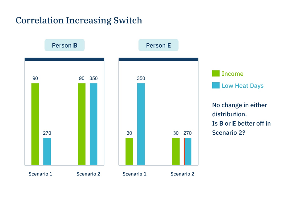
Figure 2. Judging a Change in Circumstances in a Multidimensional Setting

In Situation 1, the status quo, the matrix in Figure 1 shows that B has relatively high income ($90,000) but a high heat exposure (270 low heat days), while E has low income ($30,000) and lower heat exposure (350 cool days). There is low correlation between their rankings on the two outcomes. Imagine an alternative Situation 2 in which Person B has an income of $90,000 and heat exposure of 350 cool days, while Person E has an income of $30,000 and higher heat exposure (270 cool days). The correlation increases. It seems obvious that this change makes B better off and E worse off, increasing inequality. Their current heat stress differential (low for B high for E) was offset somewhat by income differences (high for B and low for E). In Situation 2, it the increase in correlation across dimensions increased inequality. This “correlation increasing switch” from Scenario 1 to Scenario 2 made matters worse.

This outcome only occurs because the two dimensions are substitutes for one another. Having more income offsets higher heat exposure—the person can now afford an air conditioner. If the two dimensions are complementary to one another, the correlation increasing switch will improve matters. For example, suppose the two dimensions are air quality and park acreage. A given increase in nearby park acreage is made more valuable to park users by virtue of having good outdoor air quality.

Thus, when considering how to combine column scores to evaluate a whole matrix, both the statistical correlations across the multiple column distributions and the cumulative risks associated with how these interact need to be considered. Economists have derived various generalizations of the single-column formula specified above that can be used the build in substitution across dimensions.

Welfare Measures

The multidimensional issues addressed above for inequality measures using cumulative risk and correlation across dimensions did not consider how the individuals involved might care about the dimensions. The outcomes were objectively good or bad and the only issue was how to account for all the pluses and minuses. The preferences of the persons involved were implicitly assumed to be the same.

The welfare approach looks at the list of achievements of each individual, that is, across a row, and judges it according to that person’s preferences for the various outcomes. A number is assigned to each row that represents the level of well-being achieved by each person. For example, Person D in the matrix has a row given by Z^D=(20,330,225,33), while Person E has Z^E=(4,350,330,30). A well-being index is developed for each person, with no presumption that if we switched two rows, say giving Z^E to Person D and Z^D to Person E, the well-being of each would be unchanged. The issues expand beyond the resources one has available to how well those resources match what one cares about, allowing persons to satisfy their preferences.

The challenge here is to develop individual well-being indices that can be added up across individuals. There are several ways that can be done. One way is to ask people about their level of life satisfaction and then statistically relate these self-reported satisfaction levels to objective circumstances (like those in the achievement matrix) that facilitate attainment of subjective well-being. Another is for the decision-maker to assign well-being indices to each person. Another, the equivalent income approach, works as follows. First, one picks a best possible outcome for every dimension except income. In an urban version of our example, this might be 1,000 acres of parks (New York’s Central Park is 840 acres, for reference), and 365 days each of good air quality and cool temperatures. A well-being index is the level of income that makes the person indifferent between the best possible achievements and their current achievements (except for income). Consider Person A in the example provided in Table 1. The analyst then determines by surveys the level of income Y (in thousands of dollars) that would make each person indifferent between (35,290, 250, Y) and (1,000, 365, 365, 30). The answer is a well-being index.

Each of these are ways to measure individual well-being. Then, axioms can be invoked for how to add up across persons to get an overall well-being measure summarizing the entire matrix. One can use a utilitarian approach (a simple sum) or a prioritarian one, in which transfer-like axioms result in giving priority to those worse off.

Discussion

Clearly, there was little room here for elaboration of important details and nuances. But we hope one message is clear. When embarking on an approach such as that suggested by Feltman-Frank and coauthors, which involves measurement of the amount of environmental injustice and how it may be affected by development-cum-mitigation projects, care should be devoted to the measurement task. Multidisciplinary collaborations among various bio-physical scientists, epidemiologists, public health experts, and social scientists will be needed. Then, a well-developed set of economic results relates them to a theory of measurement of social well-being. The axiomatic approach transparently allows everyone to understand the ethical judgments embodied in the analysis and to see how those judgments play out in the measurement of the amount of injustice under different project and mitigation options.